Angle Axis
Table of Contents
Rotation about the $x$-axis is a special case of a three-dimensional rotation. It can be expressed with Euler angles, but it is also naturally represented by a single angle $\theta$ and a rotation axis $\mathbf u = [1, 0, 0]^T \in \mathbb R^3$. This form is known as the angle-axis representation, where the rotation vector $\phi = \theta \mathbf u$ encodes both the axis direction and the rotation magnitude. Note that the axis vector is assumed to be normalized, $||\mathbf u|| = 1$.
This post explores the relationship between a rotation matrix and the angle-axis representation. First, we derive the rotation matrix for the simple case of rotation about the $x$-axis, and then generalize the result to an arbitrary unit axis $\mathbf u$ and angle $\theta$. We also show how the angle-axis can be recovered from a given rotation matrix.
From the angle-axis to rotation matrix
In this section, we derive a rotation matrix from the angle-axis representation. We start with the simple case of rotation about the $x$-axis, then extend the derivation to an arbitrary rotation axis and angle.
a simple case
In the simple case, $x$-axis is a rotation direction with magnitude $\theta$, new unit vectors after rotation are expressed as
$$ \begin{aligned} \mathbf e_{x'} &= \begin{bmatrix}1& 0& 0\end{bmatrix}^T \\ \mathbf e_{y'} & = \begin{bmatrix}0& \cos \theta& \sin \theta\end{bmatrix}^T \\ \mathbf e_{z'} &= \begin{bmatrix}0& -\sin \theta& \cos \theta\end{bmatrix}^T \end{aligned} $$Furthermore, these unit vectors are derived from original unit vectors, $\mathbf e_x, \mathbf e_y$ and $\mathbf e_z$,
$$ \begin{aligned} \begin{bmatrix} \mathbf e_{x'} \\ \mathbf e_{y'} \\ \mathbf e_{z'} \end{bmatrix}^T &= \begin{bmatrix} 1 \cdot \mathbf e_x + 0 \cdot \mathbf e_y + 0 \cdot \mathbf e_z \\ 0 \cdot \mathbf e_x + \cos\theta \cdot \mathbf e_y + \sin \theta \cdot \mathbf e_z \\ 0 \cdot \mathbf e_x - \sin \theta \cdot \mathbf e_y + \cos \theta \cdot \mathbf e_z \end{bmatrix}^T \\ &= \begin{bmatrix}\mathbf e_x& \mathbf e_y& \mathbf e_z\end{bmatrix}\begin{bmatrix}1& 0 & 0 \\0& \cos \theta & -\sin \theta \\0& \sin \theta & \cos \theta\end{bmatrix} \end{aligned} $$where $[\mathbf e_x\quad \mathbf e_y\quad \mathbf e_z]$ is an identity matrix.
Although the above equations already give the rotation matrix, there is another way to obtain it: multiply $[\mathbf e_{x’}, \mathbf e_{y’}, \mathbf e_{z’}]$ by $[\mathbf e_x, \mathbf e_y, \mathbf e_z]^T$, that is,
$$ \begin{aligned} \begin{bmatrix} \mathbf e_{x'}& \mathbf e_{y'}& \mathbf e_{z'} \end{bmatrix} \begin{bmatrix} \mathbf e_{x}^T\\ \mathbf e_{y}^T \\ \mathbf e_{z}^T \end{bmatrix} &= \begin{bmatrix}\mathbf e_x& \cos\theta\mathbf e_y + \sin \theta \mathbf e_z& -\sin\theta \mathbf e_y + \cos\theta \mathbf e_z\end{bmatrix}\begin{bmatrix} \mathbf e_{x}^T\\ \mathbf e_{y}^T \\ \mathbf e_{z}^T \end{bmatrix}\\ &= \mathbf e_x\mathbf e_x^T + \cos\theta \mathbf e_y\mathbf e^T_y + \sin\theta\mathbf e_z\mathbf e^T_y -\sin \theta\mathbf e_y \mathbf e^T_z + \cos\theta \mathbf e_z\mathbf e^T_z \\ &= \begin{bmatrix}1\\0\\0\end{bmatrix}\begin{bmatrix}1&0&0\end{bmatrix} + \cos\theta \mathbf e_y\mathbf e^T_y + \sin\theta\mathbf e_z\mathbf e^T_y -\sin \theta\mathbf e_y \mathbf e^T_z + \cos\theta \mathbf e_z\mathbf e^T_z \\ &= \begin{bmatrix} 1& 0& 0 \\ 0& 0& 0 \\ 0& 0& 0 \end{bmatrix} + \cos\theta \begin{bmatrix} 0& 0& 0 \\ 0& 1& 0 \\ 0& 0& 0 \end{bmatrix} + \sin \theta \begin{bmatrix} 0& 0& 0 \\ 0& 0& 0 \\ 0& 1& 0 \end{bmatrix} - \sin \theta \begin{bmatrix} 0& 0& 0 \\ 0& 0& 1 \\ 0& 0& 0 \end{bmatrix} + \cos\theta \begin{bmatrix} 0& 0& 0 \\ 0& 0& 0 \\ 0& 0& 1 \end{bmatrix} \\ &= \begin{bmatrix} 1& 0 & 0 \\ 0& \cos \theta & -\sin \theta \\ 0& \sin \theta & \cos \theta \end{bmatrix} \\ &= R(x, \theta) \end{aligned} $$arbitrary rotation vector
Now we set that specific derivation aside and consider an arbitrary rotation axis $\mathbf u\in\mathbb R^3$. Let $\mathbf v$ be a unit vector orthogonal to $\mathbf u$, and define $\mathbf w = \mathbf u \times \mathbf v$. The vectors $\mathbf u$, $\mathbf v$, and $\mathbf w$ then form an orthonormal basis. In analogy with the simple case of rotation about the $x$-axis, rotating by $\theta$ about $\mathbf u$ gives
$$ \begin{aligned} \mathbf u' &= \mathbf u \\ \mathbf v' &= \cos \theta \cdot \mathbf v + \sin \theta \cdot \mathbf w \\ \mathbf w' &= -\sin \theta \cdot \mathbf v + \cos \theta \cdot \mathbf w \end{aligned} $$which can be expressed as matrix vector multiplication
$$ \begin{bmatrix}\mathbf u'& \mathbf v'& \mathbf w'\end{bmatrix} = \begin{bmatrix}\mathbf u& \mathbf v& \mathbf w\end{bmatrix}\begin{bmatrix}1& 0 & 0 \\ 0& \cos \theta & -\sin \theta \\ 0& \sin \theta & \cos \theta\end{bmatrix} $$Then, based on these orthonormal vectors, there is a way to construct a rotation matrix1 as
$$ \begin{aligned} R(\mathbf u, \theta) &= \begin{bmatrix}\mathbf u'& \mathbf v'& \mathbf w'\end{bmatrix} \begin{bmatrix}\mathbf u^T \\ \mathbf v^T \\ \mathbf w^T\end{bmatrix}\\ &=\begin{bmatrix}\mathbf u& \mathbf v& \mathbf w\end{bmatrix}\begin{bmatrix}1& 0 & 0 \\ 0& \cos \theta & -\sin \theta \\ 0& \sin \theta & \cos \theta\end{bmatrix}\begin{bmatrix}\mathbf u^T \\ \mathbf v^T \\ \mathbf w^T\end{bmatrix} \\ &= P S P^T \end{aligned} $$Generally, considering a vector $\mathbf l = a\mathbf u + b \mathbf v + c\mathbf w$ in a three dimensional space $\mathbb R^3$, the transformation of $\mathbf l$ is
$$ \begin{aligned} PSP^T \mathbf l &= aPSP^T \mathbf u + b PSP^T\mathbf v + cPSP^T\mathbf w \\ &= aPS\begin{bmatrix}\mathbf u^T \mathbf u \\ \mathbf v^T\mathbf u \\ \mathbf w^T \mathbf u\end{bmatrix} + bPS\begin{bmatrix}\mathbf u^T \mathbf v \\ \mathbf v^T\mathbf v \\ \mathbf w^T \mathbf v\end{bmatrix} + cPS\begin{bmatrix}\mathbf u^T \mathbf w \\ \mathbf v^T\mathbf w \\ \mathbf w^T \mathbf w\end{bmatrix} \\ &= aPS\begin{bmatrix}\mathbf 1 \\ 0 \\ 0\end{bmatrix} + bPS\begin{bmatrix}\mathbf 0 \\ 1 \\ 0\end{bmatrix} + cPS\begin{bmatrix}\mathbf 0 \\ 0 \\ 1\end{bmatrix} \\ &= aP \begin{bmatrix}\mathbf 1 \\ 0 \\ 0\end{bmatrix} + bP \begin{bmatrix}\mathbf 0 \\ \cos\theta \\ \sin \theta\end{bmatrix} + cP \begin{bmatrix}\mathbf 0 \\ -\sin\theta \\ \cos \theta\end{bmatrix} \\ &= a\mathbf u + b (\cos\theta \mathbf v + \sin\theta \mathbf w) + c (-\sin\theta \mathbf v + \cos\theta \mathbf w) \\ &= a\mathbf u' + b\mathbf v' + c\mathbf w' \end{aligned} $$The above calculation shows that $PSP^T$ rotates the orthonormal basis by $\theta$ about $\mathbf u$. In other words, $PSP^T$ is the rotation matrix corresponding to the angle-axis pair $(\mathbf u, \theta)$.
obtaining rotation matrix only based $[u_1, u_2, u_3]$ and $\theta$
Although the $P$ matrix construction is valid, it is rather involved. A more convenient method is to express the angle-axis rotation as a sequence of Euler rotations. After a suitable change of basis that aligns $\mathbf u$, $\mathbf v$, and $\mathbf w$ with the $x$, $y$, and $z$ axes, the rotation by $\theta$ about $\mathbf u$ becomes a rotation by $\theta$ about the $x$-axis. The following procedure derives the rotation matrix for an arbitrary unit axis $\mathbf u$ and angle $\theta$23.
As the angle-axis representation only has the single rotation axis with $\theta$, the $x$-axis is chosen in this article.
- First rotate about the $z$-axis by $\gamma$ so that the axis $\mathbf u$ lies in the $x$-$z$ plane.
- Then rotate about the $y$-axis by $\beta$ so that $\mathbf u$ aligns with the $x$-axis.
- Perform the desired rotation by $\theta$ about the $x$-axis.
- Undo the second rotation by rotating about the $y$-axis by $-\beta$.
- Finally, undo the first rotation by rotating about the $z$-axis by $-\gamma$.
Thus, the rotation matrix can be expressed as
$$ \begin{aligned} R(\mathbf u, \theta) &= R(z, -\gamma)R(y, -\beta)R(x, \theta)R(y,\beta)R(z, \gamma) \\ &= \begin{bmatrix}\cos -\gamma& -\sin-\gamma& 0\\ \sin-\gamma& \cos-\gamma& 0\\ 0& 0& 1\end{bmatrix} \begin{bmatrix}\cos -\beta& 0& \sin-\beta\\ 0& 1& 0 \\ -\sin-\beta& 0& \cos- \beta\end{bmatrix} \begin{bmatrix}1& 0 & 0 \\ 0& \cos \theta & -\sin \theta \\ 0& \sin \theta & \cos \theta\end{bmatrix} \begin{bmatrix}\cos \beta& 0& \sin\beta\\ 0& 1& 0 \\ -\sin\beta& 0& \cos\beta\end{bmatrix} \begin{bmatrix}\cos \gamma& -\sin\gamma& 0\\ \sin\gamma& \cos\gamma& 0\\ 0& 0& 1\end{bmatrix} \end{aligned} $$Here $\cos \gamma$, $\sin \gamma$, $\cos \beta$, and $\sin \beta$ are determined from the underlying three-dimensional geometry. The order of multiplication is essential because it reflects the order of coordinate transformations.
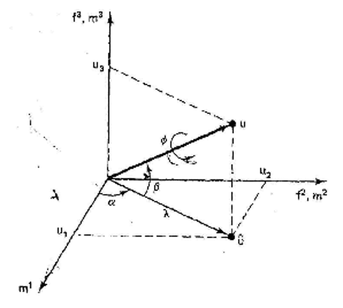
To compute these trigonometric values, consider rotating $\mathbf u = [u_1, u_2, u_3]^T$ about the $z$-axis until it lies in the $x$-$z$ plane. The transformed axis is $[u’_1, u’_2, u’_3]^T$ with $u’_2 = 0$, and it satisfies
$$ \begin{aligned} \begin{bmatrix} u'_1 \\ u'_2 \\ u'_3 \end{bmatrix} &= \begin{bmatrix}\cos \gamma& -\sin\gamma& 0\\ \sin\gamma& \cos\gamma& 0\\ 0& 0& 1\end{bmatrix} \begin{bmatrix} u_1 \\ u_2 \\ u_3 \end{bmatrix} \\ &= \begin{bmatrix} u_1\cos\gamma - u_2\sin\gamma \\ u_1\sin \gamma + u_2 \cos \gamma \\ u_3 \end{bmatrix} \end{aligned} $$Since $u’_2 = u_1\sin\gamma + u_2\cos\gamma = 0$, it is rearranged as
$$ \begin{aligned} u_1\sin\gamma &= -u_2\cos\gamma \\ \frac{\sin\gamma}{\cos\gamma} &= -\frac{u_2}{u_1} \end{aligned} $$Thus, according to the geometric relation as shown in the figure and the above equation, $\cos \gamma$ and $\sin \gamma$ are equal to
$$ \begin{aligned} \cos \gamma &= \frac{u_1}{\sqrt{u_1^2 + u_2^2}} \\ \sin \gamma &= -\frac{u_2}{\sqrt{u_1^2 + u_2^2}} \end{aligned} $$Similarly, rotating about the $y$-axis by $\beta$ aligns the axis with the $x$-axis. Using $||\mathbf u|| = 1$, we obtain
$$ \begin{aligned} \cos \beta &= \frac{\sqrt{u_1^2 + u_2^2}}{\sqrt{u_1^2+u_2^2+u_3^2}} = \sqrt{u_1^2 + u_2^2},\\ \sin \beta &= \frac{u_3}{\sqrt{u_1^2+u_2^2+u_3^2}} = u_3. \end{aligned} $$HINT:
$$u''_3 = -u'_1 \sin\beta +u'_3\cos\beta = 0$$Then, $\sin\beta / \cos\beta = u’_3 / u’_1$.
In addition, considering $||\mathbf u|| = 1$, we also have $1 = u_1^2 + u_2^2 + u_3^2$. Then, the rotation matrix can be rewritten as
$$ \begin{aligned} R(\mathbf u, \theta) &= \begin{bmatrix}u^2_1 (1 - \cos\theta) + \cos\theta& u_1u_2(1 - \cos\theta) - u_3\sin \theta& u_1u_3(1 - \cos\theta) + u_2\sin \theta\\ u_1u_2(1 - \cos \theta) + u_3\sin \theta& u^2_2(1 - \cos\theta) + \cos\theta& u_2u_3(1 - \cos \theta) -u_1\sin\theta \\ u_1u_3(1 - \cos\theta) - u_2\sin \theta& u_2u_3(1 - \cos \theta) + u_1\sin \theta & u^2_3(1 - \cos\theta) + \cos\theta \end{bmatrix} \end{aligned} $$HINT:
$$\begin{aligned}R(\mathbf u, \theta) &= R(z, -\gamma)R(y, -\beta)R(x, \theta)R(y,\beta)R(z, \gamma) \\&= \begin{bmatrix}\cos -\gamma& -\sin-\gamma& 0\\ \sin-\gamma& \cos-\gamma& 0\\ 0& 0& 1\end{bmatrix}\begin{bmatrix}\cos -\beta& 0& \sin-\beta\\ 0& 1& 0 \\ -\sin-\beta& 0& \cos- \beta\end{bmatrix}\begin{bmatrix}1& 0 & 0 \\0& \cos \theta & -\sin \theta \\0& \sin \theta & \cos \theta\end{bmatrix}\begin{bmatrix}\cos \beta& 0& \sin\beta\\ 0& 1& 0 \\ -\sin\beta& 0& \cos\beta\end{bmatrix}\begin{bmatrix}\cos \gamma& -\sin\gamma& 0\\ \sin\gamma& \cos\gamma& 0\\ 0& 0& 1\end{bmatrix} \\&= \begin{bmatrix}\cos \gamma& \sin\gamma& 0\\ -\sin\gamma& \cos\gamma& 0\\ 0& 0& 1\end{bmatrix}\begin{bmatrix}\cos \beta& 0& -\sin\beta\\ 0& 1& 0 \\ \sin\beta& 0& \cos\beta\end{bmatrix}\begin{bmatrix}1& 0 & 0 \\0& \cos \theta & -\sin \theta \\0& \sin \theta & \cos \theta\end{bmatrix}\begin{bmatrix}\cos \beta& 0& \sin\beta\\ 0& 1& 0 \\ -\sin\beta& 0& \cos\beta\end{bmatrix}\begin{bmatrix}\cos \gamma& -\sin\gamma& 0\\ \sin\gamma& \cos\gamma& 0\\ 0& 0& 1\end{bmatrix} \\&= \begin{bmatrix}\frac{u_1}{s}& -\frac{u_2}{s}& 0 \\\frac{u_2}{s}& \frac{u_1}{s}& 0 \\0& 0& 1\end{bmatrix} \begin{bmatrix}s& 0& -u_3 \\0& 1& 0 \\u_3& 0& s \\\end{bmatrix} \begin{bmatrix}1& 0 & 0 \\0& \cos \theta & -\sin \theta \\0& \sin \theta & \cos \theta\end{bmatrix} \begin{bmatrix}s& 0& u_3 \\0& 1& 0 \\-u_3& 0& s \\\end{bmatrix} \begin{bmatrix}\frac{u_1}{s}& \frac{u_2}{s}& 0 \\-\frac{u_2}{s}& \frac{u_1}{s}& 0 \\0& 0& 1\end{bmatrix} \\&= \begin{bmatrix}u_1& -\frac{u_2}{s}& -\frac{u_1u_3}{s} \\u_2& \frac{u_1}{s}& -\frac{u_2u_3}{s} \\u_3& 0& s\end{bmatrix} \begin{bmatrix}1& 0 & 0 \\0& \cos \theta & -\sin \theta \\0& \sin \theta & \cos \theta\end{bmatrix} \begin{bmatrix}u_1& u_2& u_3 \\-\frac{u_2}{s}& \frac{u_1}{s}& 0 \\-\frac{u_1u_3}{s}& -\frac{u_2u_3}{s}& s\end{bmatrix} \\&= \begin{bmatrix}u_1& -\frac{u_2}{s}\cos\theta - \frac{u_1u_3}{s}\sin\theta& \frac{u_2}{s}\sin\theta - \frac{u_2u_3}{s}\cos\theta \\u_2& \frac{u_1}{s}\cos\theta - \frac{u_2u_3}{s}\sin\theta& -\frac{u_1}{s}\sin\theta - \frac{u_2u_3}{s}\cos\theta \\u_3& s\sin\theta& s\cos\theta\end{bmatrix} \begin{bmatrix}u_1& u_2& u_3 \\-\frac{u_2}{s}& \frac{u_1}{s}& 0 \\-\frac{u_1u_3}{s}& -\frac{u_2u_3}{s}& s\end{bmatrix}\\&= \begin{bmatrix}u^2_1 + \frac{u^2_2}{s^2}\cos\theta + \frac{u_1u_2u_3}{s^2}\sin\theta - \frac{u_1u_2u_3}{s^2}\sin\theta + \frac{u^2_1u^2_3}{s^2}\cos\theta& u_1u_2-\frac{u_1u_2}{s^2}\cos\theta - \frac{u^2_1u_3}{s^2}\sin\theta - \frac{u^2_2u_3}{s^2}\sin\theta + \frac{u_1u_2u_3^2}{s^2}\cos\theta & u_1u_3+u_2\sin\theta-u_1u_3\cos\theta \\u_1u_2-\frac{u_1u_2}{s^2}\cos\theta + \frac{u^2_2u_3}{s^2}\sin\theta + \frac{u^2_1u_3}{s^2}\sin\theta + \frac{u_1u_2u^2_3}{s^2}\cos\theta& u^2_2 + \frac{u^2_1}{s^2}\cos\theta - \frac{u_1u_2u_3}{s^2}\sin\theta + \frac{u_1u_2u_3}{s^2}\sin\theta + \frac{u^2_2u^2_3}{s^2}\cos\theta & u_2u_3 -u_1\sin\theta -u_2u_3\cos\theta \\u_1u_3 - u_2 \sin\theta - u_1u_3\cos\theta& u_2u_3+u_1\sin\theta -u_2u_3\cos\theta& u^2_3+s^2 \cos\theta \end{bmatrix} \\&= \begin{bmatrix}u^2_1 + \frac{u^2_2+u^2_1u^2_3}{s^2}\cos\theta& u_1u_2(1 - \cos\theta) - u_3\sin\theta& u_1u_3 (1 - \cos\theta)+u_2\sin\theta \\u_1u_2(1 - \cos\theta) + u_3\sin\theta& u_2^2+ \frac{u^2_1+u^2_2u^2_3}{s^2}\cos\theta& u_2u_3(1 - \cos\theta)-u_1\sin\theta \\u_1u_3(1 - \cos\theta) -u_2\sin\theta& u_2u_3(1 - \cos\theta) + u_1\sin\theta & u^2_3 + (1 - u^2_3)\cos\theta\end{bmatrix}\end{aligned}$$where $s = \sqrt{u_1^2 + u_2^2}$. In addition,
$$\begin{aligned}(1 - u_1^2)(u^2_1 + u^2_2) &= (u^2_2 + u^2_3)(u^2_1+u^2_2) \\&= u^2_2u^2_1 + u^4_2+ u^2_1u^2_3 + u^2_2u^2_3 \\&= u^4_2 + u^2_2(u^2_1+u^2_3) + u^2_1u^2_3 \\&= u^4_2 + u^2_2(1 - u^2_2) + u^2_2u^2_3 \\&= u^2_2 + u^2_1u^2_3\end{aligned}$$and $u^2_1 + u^2_2u^2_3 = (1-u^2_2)(u^2_1 + u^2_2)$, so the result is calculated and simplifed by using these condition.
Now that the rotation matrix has been derived from the angle-axis, it is worth noting a simpler and more direct formula. Rodrigues’ rotation formula (also known as the Euler–Rodrigues formula) computes the matrix $R(\mathbf u, \theta)$ directly. Thus, the rotation matrix is often written as
$$ R(\mathbf u, \theta) = I +\sin\theta [\mathbf u]_\times + (1 - \cos\theta)[\mathbf u]_\times^2 $$where $[\mathbf u]_\times$ is a skew symmetric matrix introduced in Angular Velocity.
From rotation matrix to angle-axis
This section focuses on recovering the angle-axis representation from a given rotation matrix. We first extract the axis direction $\mathbf u$, then derive the rotation angle $\theta$ from the matrix.
infer $\mathbf u$
Because $\mathbf u$ lies on the rotation axis, it remains unchanged by the rotation, which means
$$ R\mathbf u = \mathbf u $$It is also unchanged by the inverse rotation, that is,
$$ R^{-1}\mathbf u = \mathbf u $$while $R^{-1} = R^T$ because of the property of rotation matrix $R$. Thus, $R\mathbf u = R^{-1}\mathbf u = R^T\mathbf u = \mathbf u$. Then, we have
$$ \begin{aligned} R\mathbf u - R^T\mathbf u &= (R - R^T)\mathbf u \\ &= \begin{bmatrix}0& r_{12} - r_{21}& r_{13} - r_{31} \\ r_{21} - r_{12}& 0& r_{23}-r_{32} \\ r_{31} - r_{13}& r_{32} - r_{23}& 0 \\ \end{bmatrix} \mathbf u\\ &= 0 \end{aligned} $$Recalling the definition of skew symmetric matrix for a vector $\mathbf a = [a_1, a_2, a_3]^T$, it is expressed as
$$ [\mathbf a]_\times = \begin{bmatrix} 0& -a_3& a_2 \\ a_3& 0& -a_1 \\ -a_2& a_1& 0 \end{bmatrix} $$Then $R - R^T$ can be viewed as the skew-symmetric matrix of a vector $\mathbf a$, and the components of $\mathbf a$ are
$$ \begin{aligned} a_1 &= r_{32} - r_{23} \\ a_2 &= r_{13} - r_{31} \\ a_3 &= r_{21} - r_{12} \end{aligned} $$Rearranging the equation of $(R - R^T)\mathbf u$ by using $[\mathbf a]_\times$, it is expressed as
$$ \begin{aligned} (R - R^T)\mathbf u &= [\mathbf a]_\times \mathbf u \\ &= \mathbf a \times \mathbf u \\ &= 0 \end{aligned} $$Thus, $\mathbf a$ is parallel with $\mathbf u$, because $\mathbf a \times \mathbf u = 0$. Then, the direction vector of $\mathbf u$ in the angle-axis representation is inferred as
$$ \mathbf u = \frac{\mathbf a}{\|\mathbf a\|} $$One may ask why $\mathbf a$ is not directly equal to $\mathbf u$. To answer this, recall the $P$ matrix representation of the rotation matrix, and express $R - R^T$ as
$$ \begin{aligned} R - R^T &= PSP^T - PS^TP^T\\ &= P(S - S^T)P^T \\ &= P\begin{bmatrix}0& 0 & 0 \\ 0& 0 & -2\sin \theta \\ 0& 2\sin \theta & 0\end{bmatrix}P^T \\ &= \begin{bmatrix} 0& 2\sin\theta \mathbf w& -2\sin\theta \mathbf v \\ \end{bmatrix} P^T \\ &= (2\sin\theta \mathbf w\mathbf v^T - 2\sin\theta\mathbf v\mathbf w^T) \\ &= 2\sin \theta (\mathbf w\mathbf v^T - \mathbf v\mathbf w^T) \end{aligned} $$when $\mathbf v = [v_1, v_2, v_3]^T$ and $\mathbf w = [w_1, w_2, w_3]^T$, the above equation is rewritten as
$$ \begin{aligned} R - R^T &= 2\sin\theta \begin{bmatrix} w_1v_1& w_1v_2& w_1v_3 \\ w_2v_1& w_2v_2& w_2v_3 \\ w_3v_1& w_3v_2& w_3v_3 \\ \end{bmatrix} - 2\sin \theta \begin{bmatrix} v_1w_1& v_1w_2& v_1w_3 \\ v_2w_1& v_2w_2& v_2w_3 \\ v_3w_1& v_3w_2& v_3w_3 \\ \end{bmatrix} \\ &= 2\sin \theta \begin{bmatrix} 0& w_1v_2 - v_1w_2& w_1v_3 - v_1w_3 \\ w_2v_1 - v_2w_1& 0& w_2v_3 - v_2w_3 \\ w_3v_1 - v_3w_1& w_3v_2 - v_3w_2 &0 \end{bmatrix} \\ &= \begin{bmatrix}0& -a_3& a_2\\ a_3& 0& -a_1 \\ -a_2& a_1& 0 \\ \end{bmatrix} \end{aligned} $$Thus, we have
$$ \begin{aligned} a_1 &= 2\sin\theta (v_2w_3 - v_3w_2) \\ a_2 &= 2\sin\theta(v_3w_1 - v_1w_3) \\ a_3 &= 2\sin\theta(v_1w_2 - v_2w_1) \\ \end{aligned} $$which can be expressed as cross product between $\mathbf v$ and $\mathbf w$1, that is
$$ \mathbf a = 2\sin\theta \mathbf v \times \mathbf w = 2\sin \theta \mathbf u $$Thus $\mathbf a$ is parallel to $\mathbf u$ and its magnitude is $2||\sin\theta||$.
infer $\theta$
Now we infer the rotation angle $\theta$ in the angle-axis representation. Using $R(\mathbf u, \theta) = PSP^T$ and the fact that similar matrices have the same trace, we obtain
$$ \begin{aligned} tr(R) = tr(PSP^T) = tr(PSP^{-1}) = tr(P^{-1}PS) = tr(S) = 1 + 2\cos\theta \end{aligned} $$Therefore,
$$ \theta = \arccos\left(\frac{\operatorname{tr}(R) - 1}{2}\right). $$Combined with $\mathbf a = 2\sin\theta,\mathbf u$, this recovers both the rotation axis and the signed angle.
HINT: $P^T = P^{-1}$
$$\begin{aligned}P^T P &= \begin{bmatrix}\mathbf u^T \\ \mathbf v^T \\ \mathbf w^T\end{bmatrix}\begin{bmatrix}\mathbf u&\mathbf v&\mathbf w\end{bmatrix} \\&= \begin{bmatrix}\mathbf u^T\mathbf u & \mathbf u^T\mathbf v& \mathbf u^T\mathbf w \\ \mathbf v^T \mathbf u & \mathbf v^T\mathbf v& \mathbf v^T\mathbf w \\ \mathbf w^T\mathbf u & \mathbf w^T\mathbf v& \mathbf w^T\mathbf w\end{bmatrix} \\&= \begin{bmatrix}1& 0& 0\\ 0&1& 0\\ 0& 0 & 1\end{bmatrix} = P^{-1}P\end{aligned}$$
special cases
Finally, note the special cases when $R = R^T$. In those cases the rotation angle is either $0$ or $\pi$. As discussed in lecture notes1, if $\theta = 0$, then
$$ \begin{aligned} R(\mathbf u, \theta) &= PSP^T \\ &= \begin{bmatrix}\mathbf u& \mathbf v& \mathbf w\end{bmatrix}\begin{bmatrix}1& 0 & 0 \\ 0& \cos \theta & -\sin \theta \\ 0& \sin \theta & \cos \theta\end{bmatrix}\begin{bmatrix}\mathbf u^T \\ \mathbf v^T \\ \mathbf w^T\end{bmatrix} \\ &= \begin{bmatrix}\mathbf u& \mathbf v& \mathbf w\end{bmatrix}\begin{bmatrix}1& 0 & 0 \\ 0& 1 & 0 \\ 0& 0 & 1\end{bmatrix}\begin{bmatrix}\mathbf u^T \\ \mathbf v^T \\ \mathbf w^T\end{bmatrix} \\ &= I \end{aligned} $$Also, the axis direction remains $\mathbf u$. If $\theta = \pi$, the rotation matrix is expressed as
$$ \begin{aligned} R(\mathbf u, \theta) &= PSP^T \\ &= \begin{bmatrix}\mathbf u& \mathbf v& \mathbf w\end{bmatrix}\begin{bmatrix}1& 0 & 0 \\ 0& \cos \theta & -\sin \theta \\ 0& \sin \theta & \cos \theta\end{bmatrix}\begin{bmatrix}\mathbf u^T \\ \mathbf v^T \\ \mathbf w^T\end{bmatrix} \\ &= \begin{bmatrix}\mathbf u& \mathbf v& \mathbf w\end{bmatrix}\begin{bmatrix}1& 0 & 0 \\ 0& -1 & 0 \\ 0& 0 & -1\end{bmatrix}\begin{bmatrix}\mathbf u^T \\ \mathbf v^T \\ \mathbf w^T\end{bmatrix} \\ &= \begin{bmatrix} \mathbf u &-\mathbf v &-\mathbf w\end{bmatrix}\begin{bmatrix}\mathbf u^T \\ \mathbf v^T \\ \mathbf w^T\end{bmatrix} \\ &= \mathbf u\mathbf u^T - \mathbf v\mathbf v^T - \mathbf w\mathbf w^T \end{aligned} $$Since $\mathbf u, \mathbf v$ and $\mathbf w$ are orthonormal basis, $\mathbf u\mathbf u^T + \mathbf v\mathbf v^T + \mathbf w\mathbf w^T = I$, then the rotation matrix is rewritten as
$$ R(\mathbf u, \theta) = 2\mathbf u\mathbf u^T - I $$So the direction vector can be derived from $R(\mathbf u, \theta) + I$ where the nonzero column is parallel to $\mathbf u$.
In conclusion, the angle-axis representation is another mathematical way to describe rotation. It can be converted into a rotation matrix or a set of Euler angles. Although the angle-axis form has special cases such as $\theta = 0$ or $\theta = \pi$, it does not suffer from gimbal lock by itself; gimbal lock may only appear after converting to Euler angles.