Homogeneous Transformation Matrices
Table of Contents
This article explains how to construct transformation matrices using the parameters obtained from the DH convention, and how to determine the spatial position and orientation of the end-effector through algebraic calculations.
Translation Matrices
First, consider a general spatial translation. The position after translation can be described as:
$$ \begin{cases} x' = x + t_x \\ y' = y + t_y \\ z' = z + t_z \end{cases} $$where $x, y, z$ represent the original position, and $t_x, t_y, t_z$ represent the translation distances along different directions. Using matrix notation, this becomes:
$$ \begin{bmatrix}x' \\ y'\\ z'\\ 1\end{bmatrix} = \begin{bmatrix}1& 0& 0& t_x\\ 0& 1& 0& t_y\\ 0& 0& 1& t_z\\ 0& 0& 0& 1\end{bmatrix}\begin{bmatrix}x \\ y\\ z\\ 1\end{bmatrix} $$The $4 \times 4$ matrix is the translation matrix $Trans(t_x, t_y, t_z)$, an augmented matrix representing affine transformation in homogeneous coordinates. Recall the translation matrices $Trans(0, 0, d_i)$ and $Trans(a_i, 0, 0)$ from the DH convention, which represent displacements of $d_i$ and $a_i$ along the $z$ and $x$ axes respectively.
Rotation Matrices
In addition to spatial translation, rotation of a point in space must also be described by matrices. Starting with rotation by $0°$ (no rotation), the rotation matrix is defined as:
$$ Rot(x, 0) = \begin{bmatrix} \cos 0°& \cos 90°& \cos 90°& 0\\ \cos 90°& \cos 0°& \cos 90°& 0 \\ \cos 90°& \cos 90°& \cos 0°& 0\\ 0& 0& 0& 1 \end{bmatrix} = \begin{bmatrix}1& 0& 0& 0\\ 0& 1& 0& 0\\ 0& 0& 1& 0\\ 0& 0& 0& 1\end{bmatrix} $$The first three rows represent the $x, y, z$ axes, while the first three columns represent the transformed $x’, y’, z’$ axes. The angle between $x$ and $x’$ is $0°$, while the angles between $x$ and $y’, z’$ are both $90°$. Comparing translation and rotation matrices, we observe that the $3 \times 3$ submatrix (formed by the first three rows and columns) describes rotation, the first three elements of the fourth column describe translation, and the rest is the augmentation for computational consistency.
Rotation around the X-axis
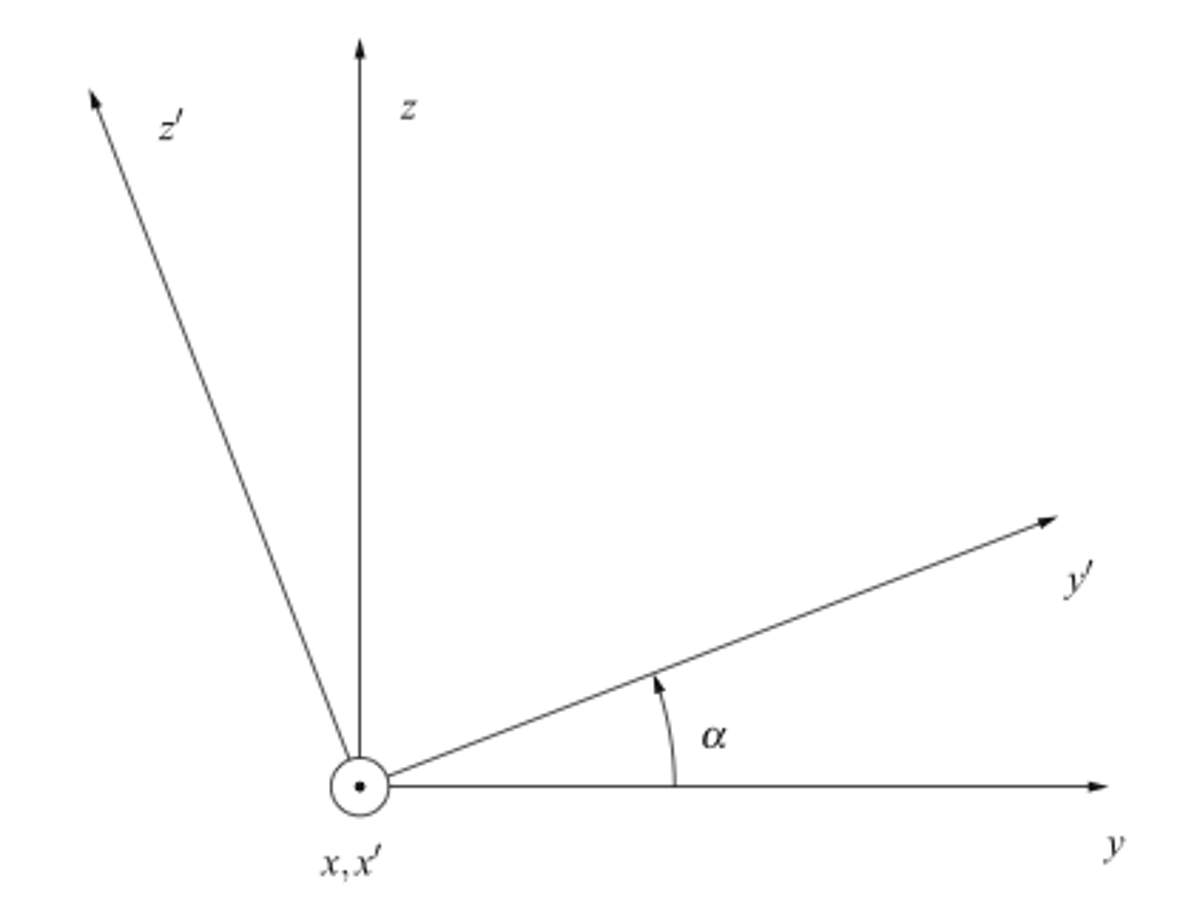
When a point rotates by angle $\alpha$ around the $x$-axis, the rotation is described as:
$$ Rot(x, \alpha) = \begin{bmatrix} \cos 0°& \cos 90°& \cos 90°& 0\\ \cos 90°& \cos \alpha& \cos (90°+\alpha)& 0 \\ \cos 90°& \cos (90°- \alpha)& \cos \alpha& 0\\ 0& 0& 0& 1 \end{bmatrix} = \begin{bmatrix}1& 0& 0& 0\\ 0& \cos \alpha& -\sin\alpha& 0 \\ 0& \sin\alpha& \cos \alpha& 0\\ 0& 0& 0& 1\end{bmatrix} $$After rotation, the relationship between the $x$-axis and the $x’, y’, z’$ axes remains unchanged. The angle between $y’$ and the original $y$, and between $z$ and $z’$, both rotate by $\alpha$. The angle between $y$ and $z’$ becomes $90° + \alpha$, while the angle between $y’$ and $z$ becomes $90° - \alpha$.
Rotation around the Y and Z axes
Similarly, rotation by $\beta$ around the $y$-axis and by $\gamma$ around the $z$-axis are expressed as:
$$ Rot(y, \beta) = \begin{bmatrix}\cos \beta& 0& \sin\beta& 0\\ 0& 1& 0& 0 \\ -\sin\beta& 0& \cos \beta& 0\\ 0& 0& 0& 1\end{bmatrix}, \quad Rot(z, \gamma) = \begin{bmatrix}\cos \gamma& -\sin\gamma& 0& 0\\ \sin\gamma& \cos\gamma& 0& 0 \\ 0& 0& 1& 0\\ 0& 0& 0& 1\end{bmatrix} $$Link Transformation Matrices
The process described above shows how to convert basic translation and rotation operations into matrices, and how the spatial relationship between two rigid bodies can be represented through such transformations. Relative to link $i-1$, the position of link $i$ is transformed by:
$$ A_{i - 1}^i = Rot(z, \theta_i)Trans(0, 0, d_i)Trans(a_i, 0, 0) Rot(x, \alpha_i) $$Forward Kinematics
Finally, based on the coordinate frames and parameters determined by the DH convention for each link, and the transformation matrices between links, we can obtain the position and orientation of the end-effector in the base space. This is achieved through matrix multiplication, mapping the end-effector information to the base frame:
$$ T = A_0^1A_1^2\cdots A_{n - 1}^n $$